American Options Pricing with a Binomial Tree

So, let's dive deeper into the model and the code. The binomial option pricing model is a very flexible tool for valuing options. It can handle certain scenarios that the black-scholes formula can't handle.

This model was first introduced in 1979 by Cox, Ross, and Rubinstein in their paper called "Option Pricing: A Simplified Approach".

Alright, let's break it down. The first thing we do is create a price tree for the underlying asset. It's like a roadmap of prices, starting from the valuation date and going all the way to the expiration date. At each step, we assume that the price of the asset will either go up or down by a certain factor.

We derive these up and down factors by utlizing the volatility of the underlying asset's price and the time it takes for each step.

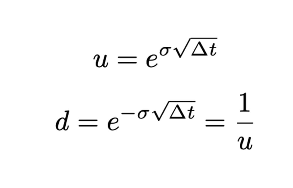
In python, numpy can be used to derive the values.

import numpy as np

"""
r = Risk Free Rate
St = Underlying Asset Price 
K = Strike/ Exercise Price
T = Time to expiration in years
sigma = Volatility of Underlying Asset's Price
q = dividend 
"""
delta_t = T/N 
u = np.exp(sigma*np.sqrt(delta_t))
d = 1/u 

Once you have the values for u and d, we are then able to calculate p, the probabiilty of the events.

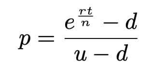
p = (np.exp((r-q)*delta_t) - d) / (u-d)

Then you will use the derive values to get the value of the underlying asset at the up nodes and down nodes as illustrated below.

As you can tell, creating the price tree for the underlying asset is pretty simple. However, as the number of steps increases, it can become quite a laborious task. But fear not, because we can make our lives easier with the help of Python. Let's take a look at how we can achieve that in the code snippet below.

 # Create an empty binomial tree for option prices
price_tree = np.zeros((N+1, N+1))
        
# Calculate the asset prices 

#Calculates the asset price at expiration
for i in range(N+1):
    for j in range(i + 1):
        price_tree[i,j] = S * u**(i - j) * d**j

#Calculate the assets prices at the other nodes. 
for j in range(N-1, -1, -1):
    for i in range(j+1):
        price_tree[i,j] = S * u**(i - j) * d**j

In the code snippet mentioned earlier, it actually starts at the terminal nodes and then goes backward. But we can tweak that code to eventually give us the option value we're looking for.

Now, let's talk about finding the option value. When we reach the expiration of the option, its value is simply its intrinsic value or exercise value, which can be determined using the formulas below:

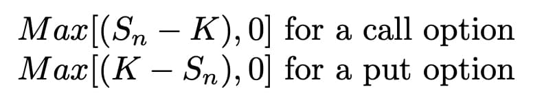
Once you've obtained the option value at the terminal nodes, the next step is to work backwards and calculate the expected value of each node. To do this, you apply the following formula:

You can achieve all of this by making some modifications to the code used for deriving the prices. Take a look at the code snippet below, which demonstrates how you can make those changes:

# Calculate the call option prices at expiration

for i in range(N+1):
    price_tree[N, i] = max(0, price_tree[N, i] - K)

# Calculate option prices at previous time steps
    for j in range(N-1, -1, -1):
        for i in range(j+1):
            exercise_value = max(0, price_tree[j, i] - K)
            continuation_value = np.exp(-r * delta_t) * (p * price_tree[j+1, i] + (1 - p) * price_tree[j+1, i+1])
            price_tree[j, i] = max(exercise_value, continuation_value)

 #Value of the Call Option                   
option_value = price_tree[0,0]

And there you have it! This code serves as a versatile framework that can be used to value various instruments that involve specific actions at different points in time, such as convertible bonds or other financial instruments. Of course, depending on the instrument, you may need to make some minor adjustments to the code, but that's something I can delve into in the future if needed.